Let's examine the following letter grade calculation:
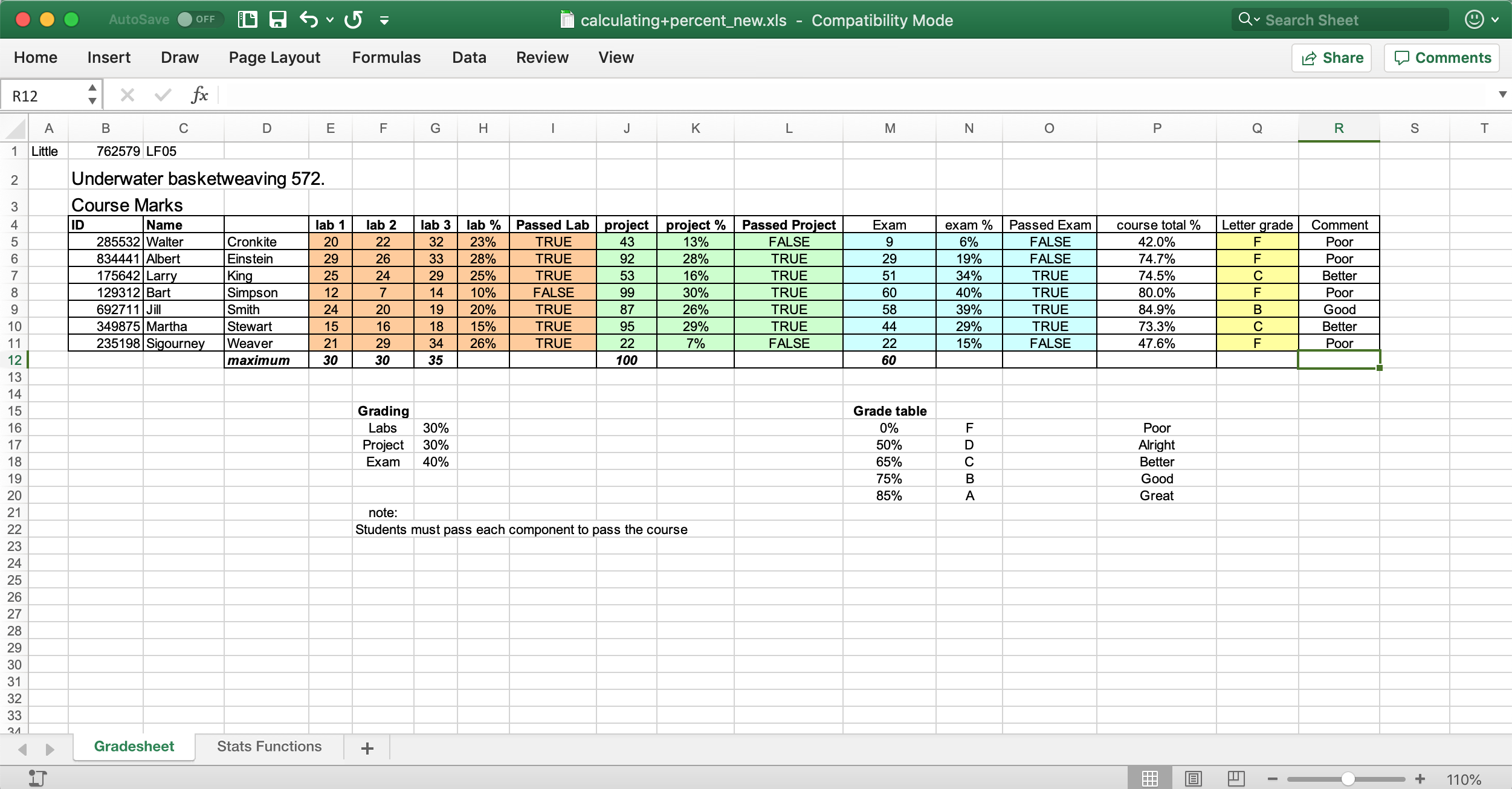
Bart Simpson (Row 8) has a course total percentage of 80% (Cell P8). He seems to have done well if you consider his course total percentage. Unfortunately, he failed the course because he failed the lab component. In the lab component he got 10%. In order to pass he needed at least 15% in the lab component.
Imagine this situation: Bart Simpson was sick while he was doing Lab 2. So, the Prof. will allow him to redo Lab 2 (obviously with a different set of lab exercises). Now, Bert Simpson wants to know what is the minimum he must get in Lab 2 in order to pass the lab component, i.e., get at least 15% marks in the lab component (Cell H8).
Excel "Goal Seek" function allows one to perform calculations like this. "Goal Seek" is part of Excel's "What-if" analysis tool. This tool is available in the "Forecast" command group of data tab.
Observe the following video to see how "Goal Seek" is performed:
Now notice the cell for Lab 2 (F8). Bert will need at least 21 out 30 if wants to pass the lab component and the course. If he gets 21 in Lab 2 then his course total percentage goes up to 84.7% and his letter grade improves to "B" from "F".
Let's consider the portfolio value calculation shown below:
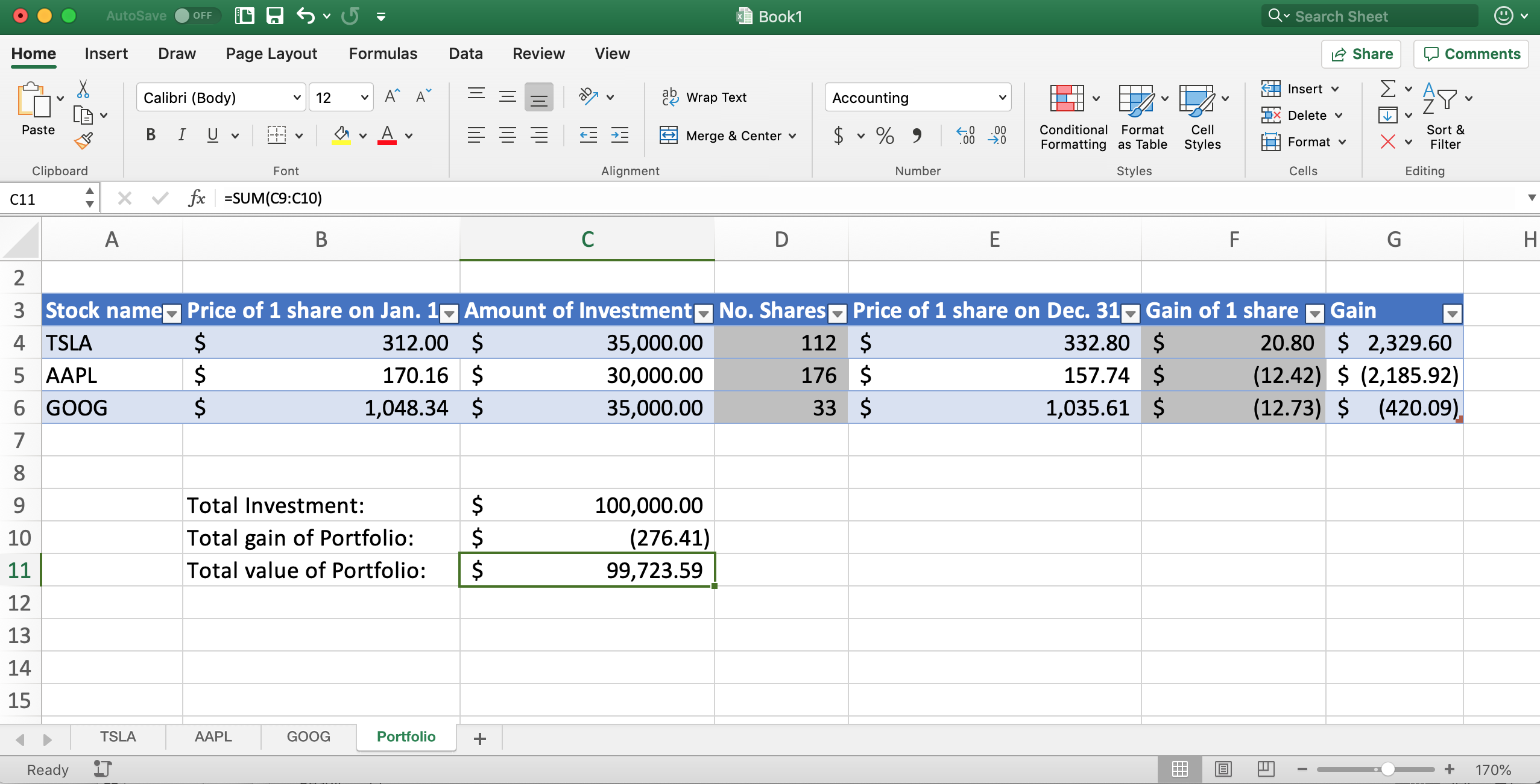
The value of the portfolio (cell C11) at the end of the year depends on the investment distribution (cells C4:C6) made at the beginning of the year.
What if the investment distribution were different in the beginning of the year. Let's say we have the following three investment distributions:
| TSLA | AAPL | GOOG |
|---|---|---|
| $25000 | $45000 | $30000 |
| TSLA | AAPL | GOOG |
|---|---|---|
| $15000 | $45000 | $40000 |
| TSLA | AAPL | GOOG |
|---|---|---|
| $40000 | $25000 | $35000 |
What would be the portfolio value in each of these investment distributions? Excel "Scenario Manager" lets you find that out. "Scenario Manager" tool is also a part of Excel's What-if Anaylysis toolbox. Observe the following video to see how "Scenario Manager" tool is used.
Among these scenarios, Scenario C yields profit on the last day of the year.
Continuing with our stock portfolio analysis, we can ask what investment distribution would have yielded the maximum portfolio value on the last day of the year. Excel's Solver tool lets us figure that out.
Excel's Solver tool is not available by default. We need to add it. Follow the steps shown in the following video to add the Solver tool. (This video is for Mac computers. A video for adding Solver for Windows computers will be shown/added later.)
Solver tool requires at least the following:
- An objective to maximize or minimize: In our stock portfolio case we wish to maximize the value of the portfolio, that is, cell C11.
- Input variables: In this portfolio value calculation, decision variables and the input variables are same.
- Decision variables: In this stock portfolio calculation, investment distribution in column C, that is, cells C4:C6 are the decision variables.
- Constraints:
- We must hold at least $10000 worth of shares for each of the stocks. That is C4:C6 ≥ 10000.
- We may not hold more than $50000 worth of shares for any of the stocks. That is, C4:C6 ≤ 50000.
- Total investment must not exceed $100000. That is, C9 ≤ 100000.
Solver tool has three methods to compute a solution:
- GRG Nonlinear: this is a nonlinear tool and one would use this tool most of the time.
- Simplex LP: if the problem is linear then one should use this tool. A global optimum can be found faster by this tool than by the other methods if ineed the problem is linear. This method will let you know whether the problem is linear or not. Since, our problem is linear we use this tool in the beginning.
- Evolutionary: The GRG Nonlinear method may "get stuck" in a local optimum solution. Evolutionary method can be used to find a better solution. Computation time is generally higher with this method.
The following video shows how to use the solver tool for the purpose of figuring out the investment distribution at the beginning of year such that the value of the portfolio is maximized at the end of the year. As the problem is linear, we first used the "Simplex LP" method then we checked whether the given solution can be improved by the other two methods. As "Simplex LP" gives the global optimum, the two other methods obviously could not improve the solution.
Some observation: A quick mental calculation tells us that the optimum investment distribution should be the following:
| TSLA | AAPL | GOOG |
|---|---|---|
| $50000 | $10000 | $40000 |
We can add more constraints and make the portfolio value calculation much more complicated than we have done here. In those complicated scenarios we will not be able to figure out the optimum investment distribution easily by any pen-and-paper calculation. We will have to rely on the Solver tool or on a similar tool.